Time Series Analysis of Malaria Trends — Burkina Faso (2016–2023)
R
Epidemiology
Malaria
DHS
climate
Time series
Quantify the trend in malaria incidence at health district level and identify the factors associated with malaria incidence in Burkina Faso from 2016-2023 using routine cases data
Author
Ousmane Diallo, MPH-PhD
Published
November 12, 2025
Project Role: Research Associate & Lead Author
Timeline: 2016-2023 Analysis Period | 2023-2024
Status: Oral presentation at ASTMH 2024 (New Orleans) | Manuscript in preparation
Overview
The aim of this study was to assess the malaria trends in Burkina Faso at the health district level to help understand the malaria transmission level between 2016 and 2023 and to determine the factors associated with malaria incidence to better understand the drivers of malaria in Burkina Faso. This analysis combined publicly available DHS/MIS and climate data with restricted HMIS surveillance data obtained from PNLP under data sharing agreement.
Role: Sole author responsible for data cleaning, quality assessment, analysis, modeling, mapping, and reporting.
Methodology Framework
Data sources & Integration
Variable
Definition
Source
Temporal
Period
Suspected cases
Clinical malaria suspicion (fever)
HMIS
Monthly
2016–2023 (excl. 2019)
Tested cases
Received RDT or microscopy
HMIS
Monthly
2016–2023
Confirmed cases
Positive RDT or microscopy
HMIS
Monthly
2016–2023
Presumed cases
Treated without positive test
HMIS
Monthly
2016–2023
Population
District population
HMIS
Annual (Monthy est)
2016–2023
Treatment-seeking (U5)
Public/private/no care
DHS/MIS
Every 3 years
2014, 2017–18, 2021
Data management
A standard data quality workflow before analysis was applied:
Standardized district and facility names across years.
Crude malaria incidence was calculated by dividing the number of reported confirmed cases for each health district and month by the district population and multiplying by 1000. Then, crude incidence was adjusted for each factor in accordance with the WHO framework.
Incidence Adjustment Framework (WHO Guidelines):
Crude: Raw confirmed cases / population × 1,000
Adjustment 1: Account for testing rate variations
Adjustment 2: Account for facility reporting completeness
Adjustment 3: Account for care-seeking behavior patterns
Statistical Analysis Methods
Time Series Decomposition
STL decomposition (LOESS) to separate seasonal, trend, residual components.
Sen’s slope for monotonic trend magnitude.
Mann–Kendall test for trend significance (α = 0.05).
View STL Decomposition Implementation
# Normalization helpergetNormalized <-function(vec) {if (!is.numeric(vec) ||all(is.na(vec))) {warning("Input vector is non-numeric or all NA; returning original vector")return(vec) } vec_mean <-mean(vec, na.rm =TRUE) vec_sd <-sd(vec, na.rm =TRUE)if (is.na(vec_sd) || vec_sd ==0) {warning("Standard deviation is 0 or NA; returning original vector")return(vec) } (vec - vec_mean) / vec_sd}monthly_DS_incidence <- monthly_DS_incide %>% dplyr::mutate(mal_cases_norm =getNormalized(`Incidence brute`),incidence_adj_presumed_cases_norm =getNormalized(Adj1),incidence_adj_presumed_cases_RR_norm =getNormalized(Adj2),incidence_adj_presumed_cases_RR_TSR_norm =getNormalized(Adj3) )
Factors associated with incidence
Model Type: Generalized Additive Models (GAMs) for non-linear relationships
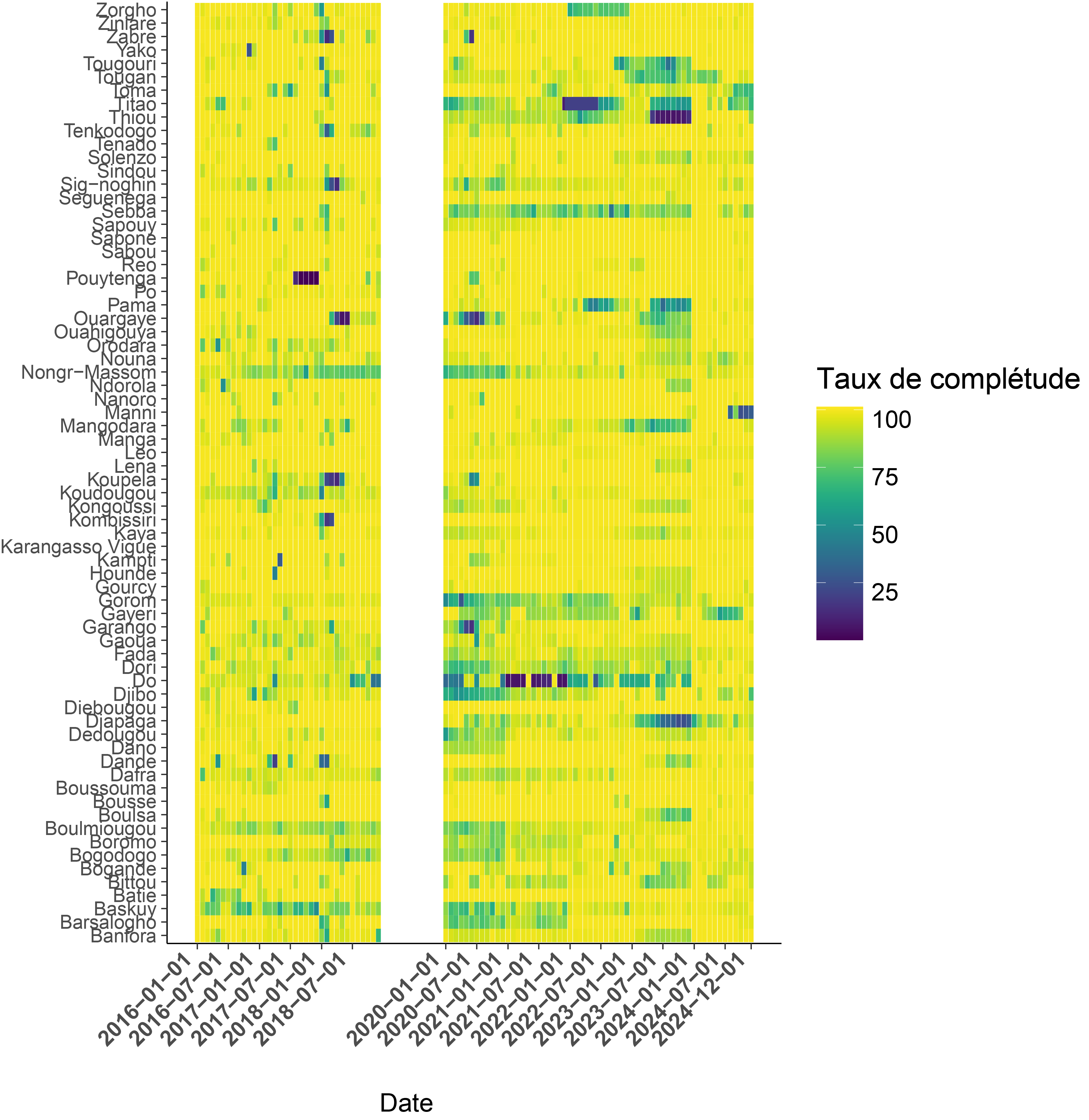
Key Insight: Reporting completeness varied dramatically (50-100% across districts), with systematic gaps that biased crude incidence estimates. This finding led to policy recommendations for surveillance system strengthening.
Burden Estimation Results
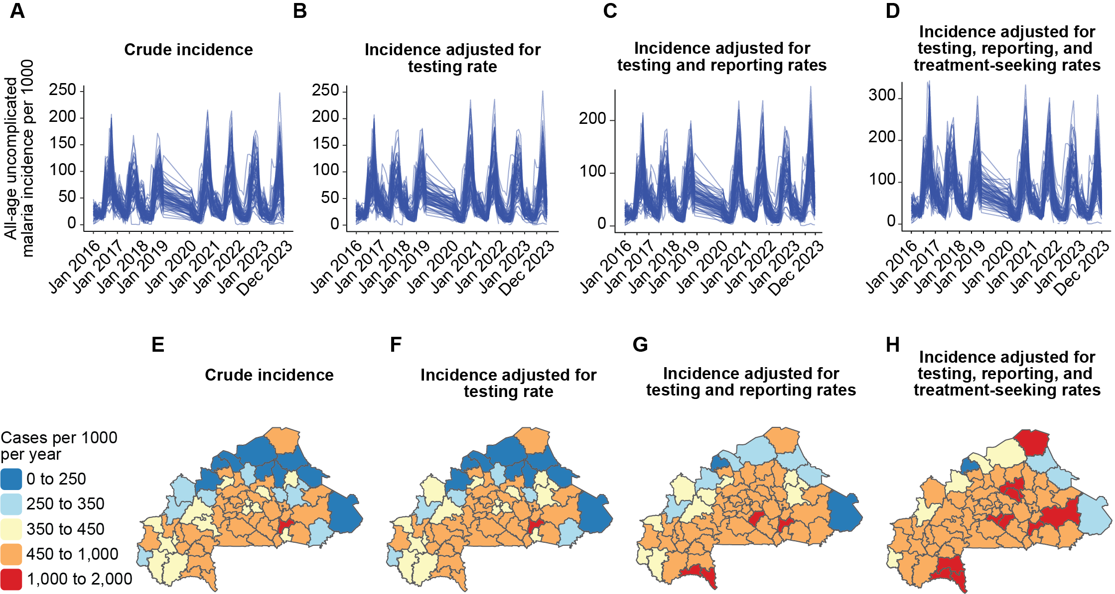
Fig. Incidence estimates following WHO framework. A-D: Temporal trend for the four incidences (crude incidence, incidence adjusted by testing rate, incidence adjusted by testing rate and reporting rate, incidence adjusted by testing rate, reporting rate and care-seeking rate; E-D: Spatial analysis for the four incidences from 2023.
Care-seeking adjustment critical: Added ~450 cases/1,000 in Gorom-Gorom, Gaoua, Kaya
Policy Impact: Demonstrated need for integrated care-seeking behavior in burden estimation
Temporal Trend Analysis
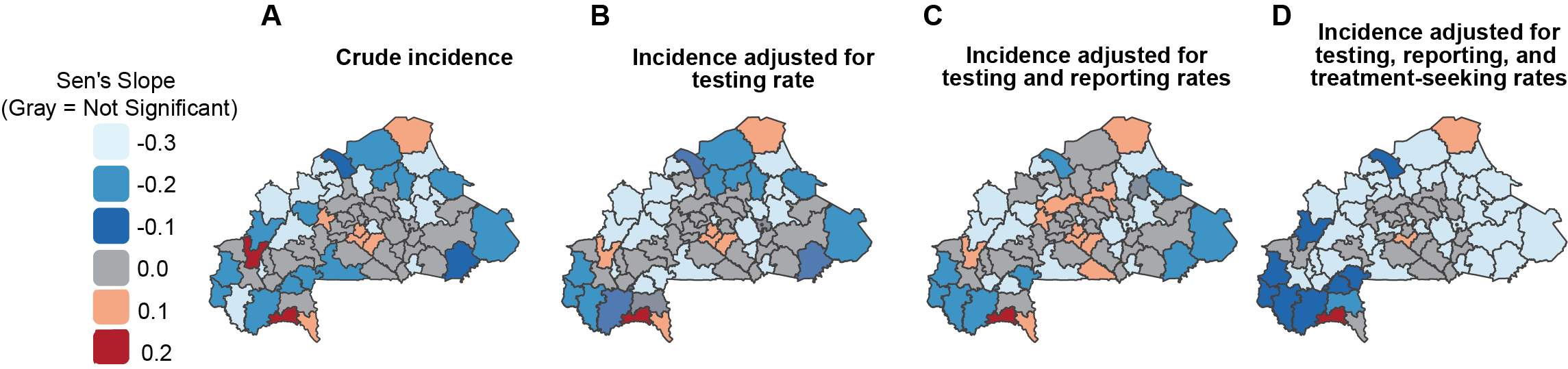
Fig. Sen’s slope coefficient for the trend of malaria incidence adjusted for testing rate, weighted reporting rate and care-seeking rate; Gray color: not significant.
Public: DHS/MIS surveys, and CHIRPS climate data are fully open-access.
Restricted: HMIS surveillance data (available under PNLP data sharing agreement).
Reproducibility: Complete analytical code provided for transparency
Collaboration & Leadership
Stakeholder Engagement:
Direct collaboration with Burkina Faso National Malaria Control Programme
World Health Organization
This project demonstrates expertise in epidemiological surveillance, advanced time series analysis, multi-source data integration, and evidence-based policy support using state-of-the-art statistical methods and reproducible research practices.
Ousmane Diallo, MPH-PhD – Biostatistician, Data Scientist & Epidemiologist based in Chicago, Illinois, USA. Specializing in SAS programming, CDISC standards, and real-world evidence for clinical research.